The phone and vehicle links in this series both operate in a medium that does nothing. Air, plastic and glass are non-magnetic and non-conducting, so the gap is an inconvenience and not a participant.

Seawater is a participant. Its conductivity is roughly 4 S/m — around eight orders of magnitude above fresh air and comparable in effect to placing a lossy conductive sheet in the middle of your coupler. Everything else about an underwater link follows from that single number.

This article works through a 500 W autonomous underwater vehicle (AUV) docking charger at 100 kHz.

Design study. Subsea equipment is governed by pressure, materials and marine-operations requirements that this article does not address. Treat the numbers as sizing exercises.

Reading route: why remove the connector → what the medium does → choosing a frequency → numbers → mechanics → docking → system issues → verification.

1. Why remove the connector

Subsea power is normally transferred through wet-mate connectors: precision-machined, oil-filled, pressure-balanced assemblies that mate underwater. They work, and they are the reason most of this equipment exists at all. They are also the component that limits several things at once.

• They are expensive relative to the vehicle, and the cost is per-mating-pair.
• Their seals are a maintenance item and a failure mode, and a flooded connector usually means a flooded electronics housing.
• They have a finite number of mating cycles, which sets an operational limit on an AUV expected to dock hundreds of times.
• Mating requires mechanical precision, which pushes complexity onto the docking system or onto ROV intervention.

An inductive link removes the electrical interface entirely. The pressure housings stay sealed for the life of the deployment, mating cycles become mechanical rather than electrical, and alignment tolerance becomes a design variable instead of a hard requirement.

That is a genuine improvement, and it is bought with a new set of problems.

2. What the medium does

The magnetic coupling itself is essentially unaffected. Seawater has \(\mu_r\approx1\), so equation (1) of the phone article holds unchanged: \(k\) measured in water is very nearly \(k\) measured in air. This is worth stating clearly because it is often assumed otherwise, and because it makes a useful diagnostic — see section 8.

What changes is loss. The time-varying magnetic field induces an electric field in the surrounding water, and because the water conducts, that field drives current:

\[\mathbf J=\sigma\mathbf E,\qquad p_{\mathrm{eddy}}=\sigma|\mathbf E|^2,\qquad |\mathbf E|\propto\omega|\mathbf B|. \tag{1}\]

Combining these, the volumetric loss in the medium scales as

\[P_{\mathrm{eddy}}\propto\sigma\,\omega^2B^2. \tag{2}\]

Two consequences follow immediately. Loss is proportional to conductivity, so fresh water is a far more forgiving medium than seawater by a factor of several hundred. And loss rises with the square of frequency, which removes the usual strategy of raising frequency to raise quality factor.

The associated length scale is the skin depth,

\[\delta=\frac{1}{\sqrt{\pi f\mu_0\sigma}}. \tag{3}\]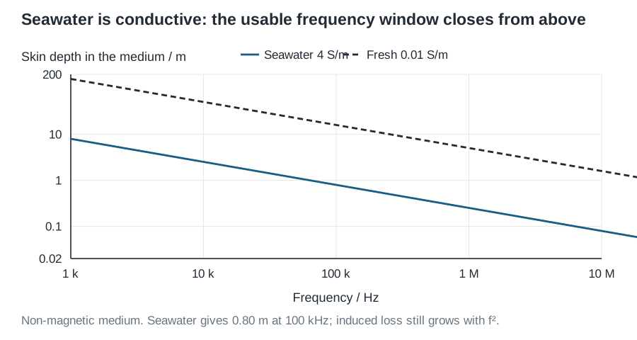

At 100 kHz in seawater δ ≈ 0.80 m, far larger than a coupler, so the field is not shielded and the induced loss is a modest fraction rather than a wall. It still grows as f² — the penalty accumulates quietly rather than appearing suddenly. Open full size

Seawater’s relative permittivity is also high, around 81. That is irrelevant to an inductive link, but it is precisely why capacitive power transfer — impractical in air at these distances — is a credible alternative underwater, and why some subsea work uses it.

3. Choosing a frequency

In air, the frequency choice is a straightforward trade: higher frequency gives higher \(Q=\omega L/R\) until winding losses catch up, so more frequency is more efficiency until it isn’t. That is how the EV case reached \(Q=356\) and rescued its weak coupling.

Underwater, a third term enters. Model the medium’s dissipation as an additional series resistance \(R_{\mathrm{med}}\) reflected into the coil, so that

\[Q_{\mathrm{eff}}=\frac{\omega L}{R_{\mathrm{coil}}(\omega)+R_{\mathrm{med}}(\omega)},\qquad R_{\mathrm{med}}\propto\sigma\omega^2. \tag{4}\]

The numerator rises linearly; the medium term in the denominator rises quadratically. There is therefore an optimum frequency, and it is lower than the air-side intuition suggests. Practical subsea inductive links generally sit in the tens to low hundreds of kilohertz, rather than the megahertz region used for small air-gap links.

The useful part of equation (4) is that it folds the whole problem back into the framework already established: the medium attacks \(Q\), and \(kQ\) still bounds the efficiency. Seawater is not a new physics problem. It is a quality-factor problem with an unusual cause.

4. Numbers for a 500 W AUV link

Take a coaxial coupler — a solenoid on the vehicle nose sliding inside a cradle winding — with \(L_1=L_2=50\ \mu\mathrm H\) at 100 kHz, so \(\omega L=31.4\ \Omega\). Coaxial geometry gives good coupling; allow \(k=0.5\) after leaving clearance for docking tolerance and fouling.

With Litz coils at \(R_{\mathrm{coil}}=0.12\ \Omega\):

\[Q_{\mathrm{air}}=262,\qquad kQ=131,\qquad \eta_{\max}=98.5\%. \tag{5}\]

Now suppose the medium contributes an equivalent \(R_{\mathrm{med}}=0.12\ \Omega\) — that is, it halves the quality factor. This is an illustrative assumption, not a measured value; the real figure depends on coupler geometry, the volume of water carrying significant field, and the shielding.

\[Q_{\mathrm{eff}}=131,\qquad kQ=65,\qquad \eta_{\max}=97.0\%. \tag{6}\]

Halving \(Q\) costs 1.5 percentage points. That is the honest headline: at these frequencies and this scale, seawater is a real but survivable loss term, not a barrier. The pressure housing and the docking mechanism are harder problems than the conductivity.

It also shows where the danger is. Push the same design to 1 MHz to shrink the magnetics and \(R_{\mathrm{med}}\) rises by a factor of a hundred while \(\omega L\) rises by ten — the term that was a footnote becomes dominant. The frequency ceiling in section 3 is not a soft preference.

5. Mechanics is the real constraint

Pressure. At 1000 m the ambient pressure is about 100 bar. Coupler windings and ferrite must either sit inside a pressure vessel, be potted in a compliant material, or run pressure-balanced in an oil-filled housing. Ferrite is brittle and fails in tension; it needs mechanical support that does not itself conduct.

Conductive housings. This is the mistake worth naming explicitly. A titanium or steel housing around the coupler is structurally attractive and electrically disastrous: it is far more conductive than seawater and sits where the field is strongest. Housings in the flux path must be non-conductive — engineering polymers, ceramics, glass-reinforced composites — with metal confined to regions the field does not reach.

Corrosion and galvanic pairs. No conductor is exposed, which removes the connector’s main corrosion path. Dissimilar materials in the cradle assembly still need the usual galvanic attention.

Biofouling and sediment. Marine growth accumulates on both coupler faces over months. It does not affect \(\mu_r\), but it acts as extra gap, and the coupling curve is steep. A link designed at its nominal gap with no margin will quietly lose capability over a deployment. Design for the fouled gap, and log coupling over time so the degradation is visible before it becomes a failure.

Thermal. One genuine advantage: water is an excellent heat sink. Coupler loss that would be a thermal design problem in air is carried away readily. The electronics inside the sealed housing get no such benefit, and remain the thermal constraint.

6. Docking geometry

A functional sequence. The important structural point is that alignment is achieved mechanically, by the cradle, before power is applied — not by a control loop working against currents and vehicle dynamics. Open full size

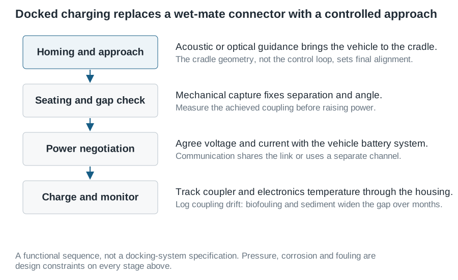
An AUV approaching a dock in a current cannot hold position to millimetres. Two strategies follow:

Let the mechanics do it. A funnel or conical cradle converts a coarse approach into a precise final position. The vehicle’s guidance only needs to get inside the capture envelope. This is the common approach and the reason coaxial couplers are popular: the vehicle drives into a ring, and the geometry enforces alignment.

Make the coupler tolerant. Rotationally symmetric couplers — a solenoid on the nose inside a cradle ring — are insensitive to roll entirely, which removes one axis from the docking problem. Arc and segmented couplers extend tolerance in pitch or yaw at some cost in coupling.

Either way, measure the achieved coupling before raising power. A low-power probe that estimates \(k\) from the reflected impedance costs nothing and prevents a badly seated vehicle from being charged at full current with an unexpected load impedance.

7. System issues

Communication. Acoustic links are slow and have long latency; optical links work well over short ranges in clear water but poorly in turbid conditions. Through a docked coupler, in-band load modulation — the same technique Qi uses — is available and reliable, because the link is already established and short. Use the coupler for the charging handshake and reserve acoustics for homing.

Safety. There is no exposed-contact shock hazard, which is the connector’s main risk removed. Stray field in water near marine life is a different and less well-characterised question; exposure guidance is written for humans in air, and applying it to a subsea installation requires judgement rather than a table lookup. Keep the field confined, and state what you assumed.

Reliability. The link’s failure modes shift from electrical (flooded connector) to mechanical (failed capture, fouled faces, cracked ferrite). This is usually a favourable trade, because mechanical degradation is gradual and observable, while a flooded connector is sudden and destroys the housing behind it. That advantage only materialises if the monitoring in section 8 is actually implemented.

8. What to verify

• Coupling in air and in water. Measure \(k\) by the open/short method in both. They should agree closely, because \(\mu_r\approx1\). A significant difference means the measurement is picking up medium loss, and tells you \(R_{\mathrm{med}}\) is larger than you assumed.
• Quality factor in situ. Measure \(Q\) in the deployment medium, at the operating frequency and temperature. This is the number equation (4) is about, and it cannot be inferred from a bench measurement in air.
• Fresh water and seawater separately. If the system may be tested in a fresh-water tank and deployed at sea, characterise both. The conductivity differs by orders of magnitude and so does the loss.
• Pressure cycling. Cycle the coupler assembly to depth repeatedly, then re-measure inductance and \(Q\). Look for ferrite cracking and potting separation.
• Fouling drift. Log \(k\) and efficiency over the deployment. A downward trend is the gap widening, and it is the main long-term degradation mechanism.
• Misaligned and no-load cases. Verify behaviour when the vehicle is partially seated, absent, or leaving mid-charge.

Across all three articles in this series, the same two numbers decide the outcome: how much flux the coils share, and how little resistance stands in the way. A phone loses coupling to a case, a car loses it to ground clearance, and an AUV loses quality factor to the sea — but \(kQ\) bounds all three.