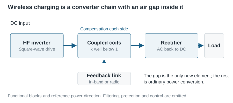
A wireless charging pad is not a new class of machine. It is a DC–DC converter whose transformer has been cut in half and separated by a few millimetres of plastic and air. Everything upstream and downstream — the inverter, the rectifier, the regulation loop — is conventional power electronics covered elsewhere in the converter series.

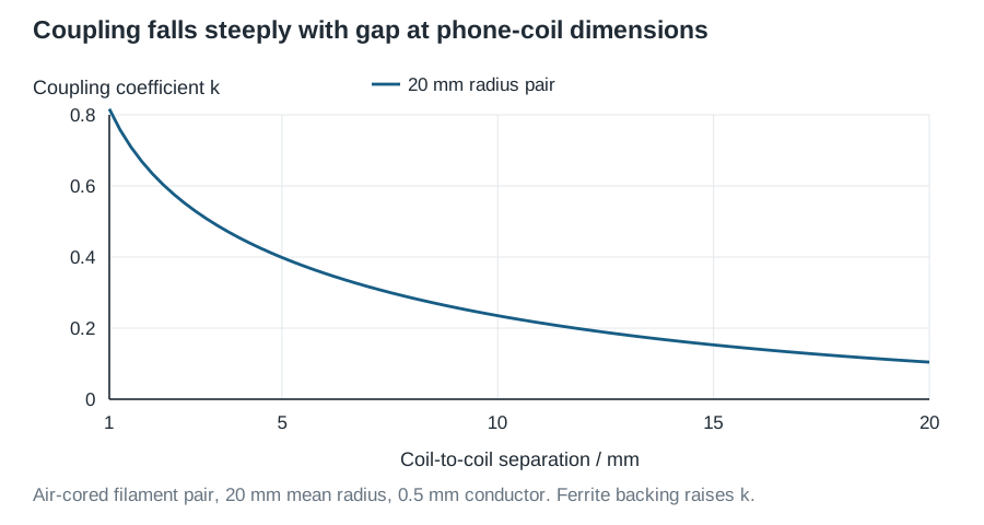
What the gap changes is the coupling. A wound transformer has a coupling coefficient above 0.99. A phone charging pad has roughly 0.3 to 0.6. That single number determines the compensation network, the control strategy, the achievable efficiency and most of the safety engineering.

This article works through a 15 W, 130 kHz link at phone dimensions.

Design study, not a certified implementation. The numbers below are analytical sizing values. Interoperable products must meet the published Qi specification, which this article does not reproduce or replace.

Reading route: the gap → compensation → the kQ limit → regulation → the protocol → foreign objects → thermal reality → what to measure.

The only unconventional element is the coupled coil pair. The feedback link exists because the quantity being regulated is on the other side of the gap. Open full size

1. What crosses the gap

Two coils share flux. The voltage induced in the secondary by primary current is

\[v_2=M\frac{di_1}{dt},\qquad M=k\sqrt{L_1L_2}, \tag{1}\]

where \(M\) is the mutual inductance and \(k\in[0,1]\) the coupling coefficient. In sinusoidal steady state at angular frequency \(\omega\), the induced EMF is \(\omega M I_1\).

Equation (1) contains the whole design problem. \(L_1\) and \(L_2\) are set by the coil you can fit in a phone; \(k\) is set by geometry you only partly control, because the user decides where the phone lands.

A filament model of two 20 mm-radius coils. Coupling roughly halves between a 3 mm and an 8 mm separation. Ferrite backing raises the absolute values; the steepness does not go away. A case, a card, or an off-centre placement all act as extra gap. Open full size

Note what is not in equation (1): the medium. Air, plastic and glass are all non-magnetic, so the coupling through a phone case is the coupling of the equivalent air gap. This stops being true in seawater, where the medium conducts.

2. Why the coils need capacitors

Drive the primary from a voltage source and the coil reactance \(\omega L_1\) opposes you directly, while only the \(\omega M\) term does useful work. At 130 kHz with \(L_1=10\ \mu\mathrm H\) and \(k=0.5\):

\[\omega L_1=8.17\ \Omega,\qquad \omega M=\omega kL_1=4.08\ \Omega. \tag{2}\]

Half the applied voltage is spent pushing current through reactance that transfers nothing. A series capacitor on each side cancels that reactance at one chosen frequency:

\[C_1=\frac{1}{\omega_0^2L_1},\qquad C_2=\frac{1}{\omega_0^2L_2}. \tag{3}\]

For \(L=10\ \mu\mathrm H\) at \(f_0=130\ \mathrm{kHz}\), \(C=150\ \mathrm{nF}\).

Series–series compensation. T1 is the coupled coil pair, not a tightly coupled transformer: its magnetising and leakage inductances are comparable. The inverter and rectifier are represented by their fundamental equivalents. Open full size · Circuit source · Drawn with AIPE-Sketch

At resonance the secondary loop presents a purely resistive load, and the primary sees a reflected resistance

\[R_{\mathrm{ref}}=\frac{(\omega M)^2}{R_2+R_L}, \tag{4}\]

where \(R_L\) is the load resistance referred to the AC side. For a bridge rectifier with a capacitive output, \(R_L=(8/\pi^2)R_{\mathrm{dc}}\).

Equation (4) explains a behaviour that surprises people: the pad’s input impedance depends on where the phone is sitting. Move the phone and \(M\) changes, so \(R_{\mathrm{ref}}\) changes quadratically. The inverter must tolerate that range, including the no-load case where \(R_{\mathrm{ref}}\) collapses to near zero.

Series–series is not the only choice. Series–parallel, LCC and hybrid networks trade load-independence, short-circuit behaviour and component count differently; the EV article works through double-sided LCC, which is the usual answer when coupling varies widely.

3. The efficiency ceiling

Define the coil quality factors \(Q_i=\omega L_i/R_i\), where \(R_i\) is the coil’s effective series resistance at the operating frequency — not its DC resistance, because skin and proximity effects dominate at 130 kHz. The maximum efficiency of the coil pair, with the load chosen optimally, is

\[\eta_{\max}=\frac{(kQ)^2}{\left(1+\sqrt{1+(kQ)^2}\right)^2},\qquad kQ=k\sqrt{Q_1Q_2}. \tag{5}\]

This is the single most useful equation in wireless power. It says that \(k\) and \(Q\) are interchangeable: weak coupling can be traded against high-quality coils. It also says the two coils are all that equation (5) describes — the inverter, rectifier and regulator losses are entirely separate.

The curve is steep below kQ ≈ 10 and nearly flat above 50. A phone link sits comfortably on the flat part; this is why the coils are rarely the dominant loss in a charging pad. Open full size

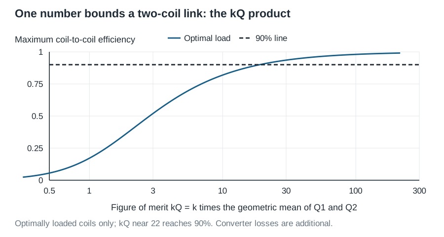
For our example, \(R_1=R_2=0.1\ \Omega\) gives \(Q=81.7\), so \(kQ=40.8\) and \(\eta_{\max}=95.2\%\).

The optimum load is \(R_{L,\mathrm{opt}}=R_2\sqrt{1+(kQ)^2}=4.08\ \Omega\). A real 15 W receiver at 12 V presents \(R_L=(8/\pi^2)(12^2/15)=7.78\ \Omega\) — nearly twice the optimum — and still achieves

\[\eta=\frac{(\omega M)^2R_L}{(R_2+R_L)^2R_1+(\omega M)^2(R_2+R_L)}=94.3\%. \tag{6}\]

The optimum is broad. Losing 0.9 percentage points for a 2:1 load error is the reason designers rarely chase it, and instead spend the freedom on regulation range.

Working the same example back through the loop gives \(I_2=1.39\ \mathrm A\) and \(I_1=2.68\ \mathrm A\) RMS, requiring an inverter fundamental of about 5.9 V RMS. A full bridge produces \((2\sqrt2/\pi)V_{\mathrm{rail}}\), so a 6.6 V rail is the minimum and a 12 V rail leaves useful control headroom. The lossless design shortcut \(I_2\approx V_1/(\omega M)\) is within a few percent here, and is a reasonable first estimate.

4. Three knobs, and where the loop closes

Battery charging needs a controlled current, then a controlled voltage. The transmitter has three ways to change delivered power:

• Frequency. Moving away from resonance detunes the network and reduces gain. Cheap, but it interacts with the compensation design and constrains the EMC picture.
• Duty or phase. Adjusting the bridge changes the fundamental amplitude. Preserves the resonant operating point but can lose soft switching at the extremes.
• Rail voltage. A preceding buck stage scales everything linearly. Clean, at the cost of another converter.

The awkward part is not the actuator but the sensor placement: the quantity to regulate is on the far side of the gap. The receiver measures it, and reports back. That is why a charging pad needs a communication channel at all, and why its control bandwidth is limited by the packet rate rather than by the power stage.

Receivers usually add local post-regulation as well, which decouples the battery charger from the slow link at the cost of another conversion.

5. The protocol does more work than the power stage

A simplified view of the session. Phase names and packet definitions belong to the Qi specification; the point here is that the pad spends most of its life in the first phase, waiting. Open full size

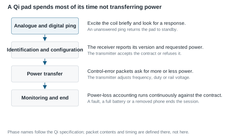
The Qi specification defines the handshake that makes any receiver work on any pad. A few structural points matter to a designer:

• The pad idles, pinging periodically. Standby power — not conversion efficiency — dominates its annual energy use.
• The receiver reports what it wants; the transmitter agrees a power contract. Everything afterwards is checked against that contract.
• Communication is in-band: the receiver modulates its load, the transmitter detects the resulting amplitude change. This is slow and shares the power path, which is why it is rugged but low bandwidth.
• Baseline power (5 W) and extended power (15 W) profiles differ in the negotiation and in the detection requirements, not in the underlying physics.
• Qi2’s magnetic profile adds alignment magnets. That is a coupling fix, not a protocol fix: it moves \(k\) up the steep part of the curve in section 1 and holds it there.

6. Foreign object detection is the hard problem

Put a coin on the pad. It sits in the same field the receiver uses, eddy currents circulate in it, and it heats. Nothing in the power path objects — the pad simply sees a slightly different load.

Two detection principles are used:

Power-loss accounting. The transmitter knows what it sent; the receiver reports what it got; the difference should match the expected link loss. Declare a fault if it does not.

Quality-factor measurement. Before power transfer, ring the coil and measure \(Q\). A lossy metal object in the field lowers it.

Both are hard for the same arithmetic reason. Consider our 15 W link at 94% coil efficiency: roughly 0.9 W is expected loss. A coin absorbing 300 mW will reach an uncomfortable temperature, but 300 mW is a 2% error on a 15 W budget — within the combined tolerance of two power measurements taken on opposite sides of a gap, calibrated independently, at unknown temperature.

This is why detection thresholds are specified rather than left to the designer, why the calibration step exists in the protocol, and why the problem gets harder as power rises — at 15 W the margin is thinner than at 5 W, with the same absolute hazard.

7. Where the heat goes

End-to-end pad-to-battery efficiency for a good 15 W system is roughly 70–80%. Coil loss is a minority share; inverter, rectifier, receiver regulation and standby account for most of it.

The thermal problem is not total loss but location. The receiver’s losses are dissipated inside the phone, millimetres from a lithium cell whose charge acceptance falls as it warms. A pad that delivers more power into a hot phone can charge it more slowly, because the battery management system throttles current. This is why bench efficiency figures and observed charging times often disagree, and why some pads include a fan.

Practical consequences: keep receiver-side loss down even at the expense of transmitter-side loss; place the coil so its loss does not sit on the cell; and measure charging performance thermally soaked, not from cold.

8. What to measure

• Coupling. Measure the primary inductance with the secondary open and shorted, then \(k=\sqrt{1-L_{\mathrm{sc}}/L_{\mathrm{oc}}}\). Sweep it over the placement envelope, not just at the aligned position.
• Quality factor. Measure at the operating frequency with an impedance analyser, at the temperature of interest. A DC resistance measurement will mislead you by a large factor.
• Efficiency. Measure at DC ports on both sides, with the receiver in a defined load state. Quote the placement.
• Standby. Measure idle input power with no receiver present, and multiply by 8760 hours.
• Temperature. Soak, then measure the receiver-side hot spot and the cell temperature. Include the foreign-object cases the specification requires.

The EV article takes the same framework to a 150 mm gap, where \(k\) falls by a factor of five and the compensation network has to change in response.