
Take the phone charging link, multiply the power by a factor of five hundred, and increase the gap from three millimetres to a hundred and fifty. The physics does not change. Almost every engineering decision does.
The dominant consequence is that the coupling coefficient falls from roughly 0.5 to roughly 0.15. Weak coupling is not a small perturbation: it changes which compensation network makes sense, it makes alignment a system-level problem rather than a user-experience one, and it means the stray field is large enough that detecting a cat under the car becomes a safety requirement.
This article works through a 7.7 kW, 85 kHz link at a 150 mm gap.
Design study, not a compliant design. Interoperable EV wireless charging is governed by published standards — SAE J2954 and the IEC 61980 series — which define geometry, test methods, field limits and detection requirements. Nothing here substitutes for them.
Reading route: what scaling breaks → the standardised operating point → why SS is not enough → LCC → misalignment → numbers → detection and fields → dynamic charging → verification.
1. What scaling breaks
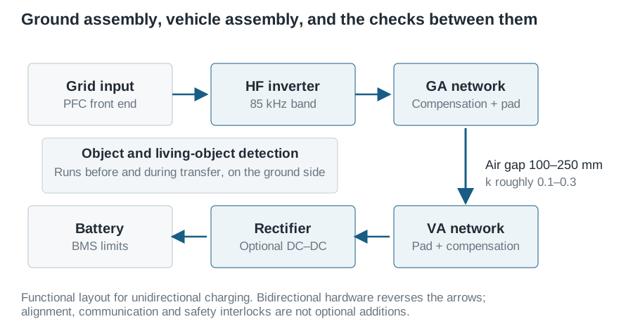
Three things change at EV scale:
Coupling collapses. At a 150 mm gap with pads of roughly 350 mm diameter, \(k\) is typically 0.1–0.3. From equation (1) of the phone article, \(M=k\sqrt{L_1L_2}\), so the useful term in the link shrinks while the coil reactance does not.
Currents become structural. Tens of amperes RMS circulate in the coils. Litz construction, capacitor RMS current ratings and pad thermal design stop being details.
The stray field escapes. A phone pad’s field is confined by the phone. A 350 mm pad radiating across 150 mm produces measurable field beyond the vehicle footprint, which brings exposure limits into the design loop.
2. The standardised operating point
Interoperability requires agreement on frequency, power class and geometry. SAE J2954 fixes:
- Frequency: a nominal 85 kHz, within an 81.38–90 kHz band.
- Power classes: WPT1 (3.7 kVA), WPT2 (7.7 kVA), WPT3 (11.1 kVA).
- Ground clearance classes: Z1, Z2 and Z3, spanning roughly 100–250 mm of vehicle-assembly height.
- Alignment tolerance: on the order of ±75 mm laterally and ±100 mm longitudinally.
The 85 kHz choice is a compromise, not an optimum. Higher frequency raises \(Q\) and shrinks magnetics, but increases switching loss, capacitor stress and EMC difficulty; lower frequency does the reverse and makes the pads impractically large. The band sits in a region that was available for this allocation.
The class structure matters more than it looks. A vehicle with a Z3 clearance and a Z1 ground pad has a much larger gap than either was designed for, so the link must be specified over a coupling range, never at a point.
3. Why series–series stops being the obvious choice
For a series–series network at resonance, the secondary current is
\[I_2=\frac{V_1}{\omega M}, \tag{1}\]which is independent of load — attractive, because it gives a natural current source for battery charging.
The problem is the denominator. \(M\) varies with parking position and vehicle height, so equation (1) makes the output current vary with where the car stopped. Worse, as \(M\to0\) the implied current diverges: an unloaded or badly aligned link drives the primary towards a short-circuit condition unless the control system intervenes.
Series–series also leaves the inverter current coupled to the load. In the phone case that was tolerable. At 7.7 kW, with \(R_{\mathrm{ref}}=(\omega M)^2/(R_2+R_L)\) swinging by an order of magnitude across the alignment envelope, it is not.
4. Double-sided LCC
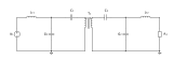
Tune each side so that
\[\omega L_{f1}=\frac{1}{\omega C_{f1}},\qquad \omega\left(L_1-L_{f1}\right)=\frac{1}{\omega C_1}, \tag{2}\]and symmetrically on the secondary. Under equation (2) the primary coil current becomes
\[I_1=\frac{V_1}{\omega L_{f1}}, \tag{3}\]which depends on neither the load nor the coupling. The output current follows as
\[I_{\mathrm{out}}\propto\frac{M\,V_1}{\omega^2L_{f1}L_{f2}}, \tag{4}\]so delivered power is proportional to \(M\) rather than inversely proportional to it.
This inverts the failure mode. With series–series, losing alignment demands more current. With LCC, losing alignment simply delivers less power at unchanged coil current — the link degrades instead of running away. That property, more than efficiency, is why double-sided LCC became common for EV charging.
The cost is real: two extra inductors carrying full coil current, two extra high-current capacitors, and a tuning condition in equation (2) that must hold across temperature and component tolerance. Detuning shows up as reactive loading on the inverter and as lost soft switching.
5. Alignment
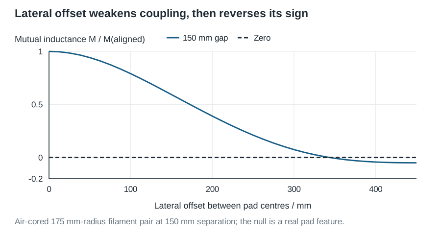
Two features of the curve drive design:
The tolerable region is a plateau, not a point. Within about ±75 mm, \(M\) falls by roughly 12%, which a controller absorbs easily. This is why the standard’s tolerance is achievable with ordinary parking.
There is a null. At large offset the coupling passes through zero and reverses. A control loop that responds to falling power by increasing excitation will drive hard into a region where no increase helps. Alignment must be measured and gated, not inferred from delivered power.
Pad geometry is the main lever. Circular pads are symmetric and simple. Polarised geometries — DD, DDQ, bipolar — produce a flux path that arcs out of the pad rather than looping locally, which raises coupling at the same gap and widens tolerance along one axis, at the cost of a more directional stray field. The choice interacts with the shielding and the field measurements in section 7.
6. Numbers for a WPT2 link
Take \(L_1=L_2=100\ \mu\mathrm H\) at 85 kHz, so \(\omega=5.34\times10^5\ \mathrm{rad/s}\) and \(\omega L=53.4\ \Omega\). With \(k=0.18\):
\[M=kL=18\ \mu\mathrm H,\qquad \omega M=9.61\ \Omega. \tag{5}\]Litz coils with \(R=0.15\ \Omega\) at the operating frequency give \(Q=356\), so
\[kQ=64,\qquad \eta_{\max}=96.9\%. \tag{6}\]Note what this says: weak coupling is not the barrier to efficiency. \(k\) fell by a factor of three from the phone case, but \(Q\) rose by more than four, and the product improved. The coil pair is not the problem at EV scale — as the kQ curve shows, everything above \(kQ\approx50\) is on the flat part.
Sizing the LCC from equation (3) with \(L_{f1}=30\ \mu\mathrm H\) (\(\omega L_{f1}=16.0\ \Omega\)) and a 600 V DC link, a full bridge gives \(V_1=540\ \mathrm V\) RMS fundamental, so
\[I_1=\frac{540}{16.0}=33.7\ \mathrm A_{\mathrm{rms}},\qquad I_2=\frac{P}{\omega MI_1}=\frac{7700}{9.61\times33.7}=23.8\ \mathrm A_{\mathrm{rms}}. \tag{7}\]Coil conduction loss is then \((33.7^2+23.8^2)\times0.15=255\ \mathrm W\), giving 96.8% across the coils — consistent with equation (6).
The remaining loss is everywhere else: compensation inductors carrying the same 34 A, capacitor ESR at tens of amperes, the inverter, the rectifier, and the PFC front end. Grid-to-battery efficiency of 90–93% for a well-aligned WPT2 link is a realistic target, and the gap between that and 96.8% is where the engineering effort actually goes.
7. Detecting what should not be there
Two distinct problems, often conflated:
Foreign object detection (FOD) addresses conductive objects in the gap — a coin, a can, a tool. Eddy-current heating in a small metal object can exceed 200 °C. The absolute hazard is the same as in the phone case, but the arithmetic is far worse: a few watts absorbed by a coin is a fraction of a percent of 7.7 kW, well inside power-measurement uncertainty. Power-loss accounting alone is therefore insufficient at this scale, and dedicated sensing — arrays of small sense coils under the pad surface, looking for local field perturbation — is the usual answer.
Living object protection (LOP) addresses animals or limbs entering the region around the pads. This is a different sensor problem: the object is larger, mostly non-conductive, and outside rather than inside the gap. Radar, capacitive sensing and cameras are all used.
Field exposure is a third, separate requirement. ICNIRP’s 2010 general-public reference level for magnetic flux density in the 3 kHz–10 MHz range is 27 µT RMS, and standards define where around the vehicle this must be met. Meeting it constrains pad geometry, shielding, and the misalignment range over which full power is permitted — a badly aligned link both delivers less power and leaks more field.
These three requirements pull against efficiency and against each other. A sense-coil array adds loss in the gap; shielding adds eddy loss; a polarised pad that improves coupling can worsen the field profile on one axis.
8. Dynamic charging
Charging while driving removes the range constraint entirely, and has been demonstrated on instrumented test tracks and short public sections.
The engineering difficulties are structural rather than electrical. A track of embedded coils must be segmented and individually energised, because energising unoccupied track wastes power and radiates. Each segment couples to the vehicle for a fraction of a second, so detection, handshake and power ramp must complete within that window, repeatedly. The civil cost of installing and maintaining power electronics under a road surface dominates the economics, and the failure mode of a buried converter is expensive.
It is a real research area with real demonstrations. It is not, at present, a deployed alternative to stationary charging, and it is worth being explicit about that distinction.
9. What to verify
- Coupling across the envelope. Measure \(k\) by the open/short method over the full lateral, longitudinal and height range, including the worst legal combination of GA and VA classes.
- Tuning under temperature. Check equation (2) holds as the compensation capacitors warm. Report the resulting inverter phase angle, not just the capacitance.
- Soft switching at the extremes. Verify at minimum and maximum coupling, minimum and maximum battery voltage, and during ramps.
- Detection performance. Test the specified objects at the specified positions, including at reduced power where the relative signal is smallest.
- Field measurement. Measure at the standard’s defined points, at worst-case alignment, at full power.
- Efficiency at DC ports. Grid input to battery terminals, with alignment and battery state stated. Anything else is a coil measurement wearing a system label.
The underwater article takes the same link into a medium that conducts, where the quality factor — the quantity that rescued efficiency here — is the thing under attack.