
A high-precision, air-cored current transducer printed directly on a PCB — wide bandwidth, no saturation, and repeatable geometry for validation, monitoring and control. This page covers how it works, why the coil shape matters, and how ours is built.
A Rogowski coil is a toroidal winding with an air core wrapped around the conductor it measures. With no magnetic material, it never saturates, stays linear from a few amps to many kiloamps, and adds almost no impedance to the circuit under test. Building it on a PCB makes every turn geometrically identical, so sensitivity is repeatable and stray-field rejection is far better than a hand-wound coil.
Our reference board integrates the coil, an active integrator and output conditioning on a single PCB, giving a ready-to-probe current output for double-pulse tests, converter validation and switching-loss measurement.
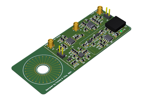
The coil responds to the rate of change of current, and an integrator turns that back into a current reading.
Ampère's law relates the magnetic field around a conductor to the current it carries. A Rogowski coil is a uniform winding of \(N\) turns forming a closed toroid around that conductor. The changing magnetic field links the turns, and by Faraday's law the coil produces an electromotive force proportional to how fast the current changes:
Here \(M\) is the mutual inductance between the coil and the conductor, \(A\) is the cross-sectional area of one turn, \(\ell = 2\pi r\) is the mean magnetic path length and \(\mu_0\) is the permeability of free space. Because the core is air, \(M\) depends only on geometry — that is the source of the coil's linearity and its immunity to saturation.
The raw output is proportional to \(di/dt\), so to recover the current itself the signal is integrated. With an active (op-amp) integrator of input resistance \(R_i\) and feedback capacitance \(C_i\), the conditioned output becomes proportional to the current, and the transducer sensitivity is:
At very high frequencies the coil can instead be operated in self-integrating mode: if it is terminated in a resistor \(R\) small compared with its own reactance (\(R \ll \omega L_c\)), the coil's inductance performs the integration and the voltage across \(R\) is already proportional to the current. Practical wideband probes combine both regimes.
No saturation, wide linear dynamic range, very wide bandwidth, negligible insertion impedance, inherent galvanic isolation, light and thin.
It cannot measure DC (it needs \(di/dt\)), the output must be integrated, and a poorly shaped coil is sensitive to conductor position and to nearby currents.
Switching-current and \(di/dt\) capture in converters, double-pulse and short-circuit tests, protection and metering, and busbar current monitoring.
Two rows of vias and the copper traces between them form the toroidal turns; the layout is what makes the sensor accurate.
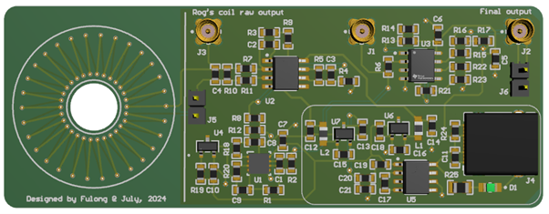
Each turn is made from a radial trace on the top copper layer, a via down to the bottom layer, a return trace, and a via back up — repeated around the aperture. An inner ring of vias and an outer ring define the winding, and the number of via pairs sets the turn count \(N\). Because a photo-plotted PCB places every via and trace to a few micrometres, all turns enclose almost exactly the same area, so the sensor's sensitivity is consistent from board to board.
A single loop of \(N\) turns going once around the toroid also forms one large loop around the toroid axis. That parasitic loop would pick up any changing field passing through the whole coil — including from nearby conductors. To cancel it, the winding is closed with a return turn: the signal is brought back through the centre of the toroid (a concentric return trace) so the net enclosed area of that outer loop is zero. Good return-path symmetry is the single most important factor in rejecting external fields and in making the reading independent of where the conductor sits inside the aperture.
Sensitivity scales with \(N\) and turn area \(A\). But more turns raise coil inductance and lower the self-resonant frequency, trading bandwidth for sensitivity.
Equal angular spacing makes the response independent of conductor position and rejects currents outside the loop. Uneven turns create position error.
A concentric return trace, or a second counter-wound layer, cancels the net enclosing loop and suppresses response to uniform external and \(dv/dt\)-coupled fields.
The aperture shape and the way the turns are drawn set the trade-off between sensitivity, bandwidth, field rejection and mechanical fit.
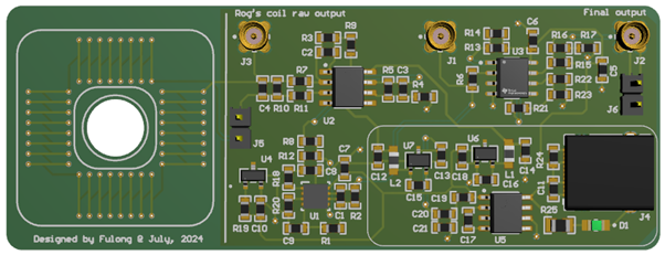
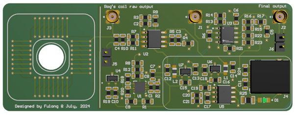
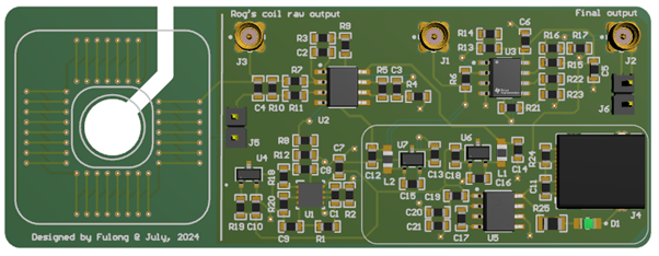
A circular aperture gives the most uniform field around the winding and the lowest sensitivity to where a round conductor sits inside it — the natural choice for cables and round busbars. A rounded-rectangular (racetrack) aperture fits flat busbars, module terminals and wide PCB tracks; the field is slightly less uniform near the corners, so turn spacing has to be managed carefully there, but it is far more practical for real power-module geometry.
The trace pattern between the two via rings is where most of the design creativity lives:
| Pattern | How it is drawn | Strengths | Trade-offs |
|---|---|---|---|
| Radial spoke | Straight radial traces between an inner and outer via ring. | Simple, highly uniform, easy to make repeatable; predictable sensitivity. | Turn density limited by via pitch on the inner ring. |
| Fishbone / herringbone | Turns tilted like a fish skeleton, alternating angle around the loop. | Packs more turns for a given radius, and the alternating tilt helps balance the return loop, improving external-field rejection. | Slightly more complex geometry; angle must stay symmetric or it adds position error. |
| Spiral / clover | Each turn spirals slightly, or the aperture is lobed. | Fits awkward mechanical openings and can raise coupling for a given footprint. | Field uniformity harder to guarantee; needs careful modelling. |
| Differential / counter-wound | Two opposing windings (or two layers wound in opposite senses) read the same current. | Strong rejection of external fields and \(dv/dt\)-coupled common-mode noise; excellent for noisy converters. | Roughly twice the layout area and complexity for the same aperture. |
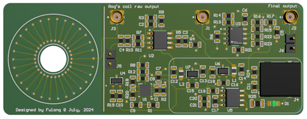
The boards below are variants of the same reference platform — the coil geometry on the left changes while the integrator and conditioning chain on the right stay common. They illustrate how aperture shape and turn density are traded against the target application.
Every geometric choice pulls on the same handful of specifications.
Rises with turn count \(N\), turn area \(A\) and smaller mean radius \(r\), since \(M \propto NA/r\). Denser windings and tighter apertures read more volts per amp.
The low end is set by the integrator; the high end by coil self-resonance \(f_r = 1/(2\pi\sqrt{L_c C_c})\). Fewer turns and shorter loops push resonance — and usable bandwidth — higher.
Uniform turns plus a symmetric return loop reject nearby currents and uniform fields. Fishbone and counter-wound patterns are chosen when the environment is electrically noisy.
A uniform, symmetric winding gives nearly the same reading wherever the conductor sits in the aperture. Non-uniform turns or corner crowding in a racetrack add position error.
Fast switching couples capacitively into the coil. A guarded, differential or counter-wound layout cancels that common-mode injection so the current signal stays clean.
Aperture shape and size are dictated by the conductor: round for cables, racetrack for busbars. The largest aperture that still couples enough flux is usually the right call.
Turning the geometry into a usable instrument means designing the electronics and calibration around it.
An active integrator sets the low-frequency limit and DC-stabilising feedback prevents output drift. Its RC time constant trades low-frequency droop against noise gain.
Damping the coil controls the self-resonant peak and keeps the phase response flat across the band, avoiding ringing on fast edges.
Low-sensitivity coils need low-noise front ends. A grounded guard ring and careful reference routing keep capacitive pickup out of the signal.
Because sensitivity is geometric, each variant is calibrated once against a reference, and the mild temperature coefficient of the integrator components is characterised.
| Parameter | Typical reference value |
|---|---|
| Aperture | Circular ~20–40 mm, or racetrack for busbars (custom on request) |
| Turns | ~40–120, set by via pitch and pattern |
| Sensitivity | Configurable via the integrator (e.g. a few mV/A after conditioning) |
| Bandwidth | Sub-kHz low corner to tens of MHz, depending on integrator and damping |
| Peak current | No saturation limit — from amps to kiloamps |
| Output | Buffered voltage on SMA/coax, integrator on board |
| Isolation | Inherent — no galvanic connection to the primary |
Values above describe the design envelope for orientation. Final specifications depend on the selected aperture, winding pattern and integrator, and are confirmed at calibration for each build.
We have designed, fabricated and bench-verified the PCB Rogowski coil boards shown above, with the coil, active integrator and output conditioning integrated on a single PCB. A demo unit is ready to ship so you can evaluate it on your own switching waveforms.
Demo units in stock · custom variants ~one month lead time.