A balanced three-phase waveform changes continuously in time. A controller can instead observe that waveform from coordinates rotating at the same speed: its fundamental then becomes constant. This is the purpose of dq modelling. It changes the description, not the physical circuit.

This companion supplies the conventions used in the SST input stage and output inverter. The derivation assumes a three-wire system without zero-sequence current; unbalanced and harmonic cases are discussed after the balanced model.

1. Define the three phases and their amplitudes

Let a positive-sequence balanced quantity have peak amplitude X and phase angle θ:

\[x_a=X\cos\theta,\qquad x_b=X\cos(\theta-2\pi/3),\qquad x_c=X\cos(\theta+2\pi/3). \tag{1}\]

Its phase RMS value is \(X/\sqrt2\), not X. A balanced line-to-line RMS voltage is \(\sqrt{3/2}X\). Consequently, the series’ 48 V line-to-line RMS input corresponds to a 39.19 V peak dq voltage; its 24 V output corresponds to 19.60 V.

2. Project onto two stationary axes

Define the amplitude-invariant Clarke transform:

\[\begin{bmatrix}x_\alpha\\x_\beta\end{bmatrix} =\frac23 \begin{bmatrix}1&-1/2&-1/2\\0&\sqrt3/2&-\sqrt3/2\end{bmatrix} \begin{bmatrix}x_a\\x_b\\x_c\end{bmatrix}, \qquad x_0=\frac{x_a+x_b+x_c}{3}. \tag{2}\]

Substituting the balanced waveforms gives \(x_\alpha=X\cos\theta\) and \(x_\beta=X\sin\theta\). The factor 2/3 preserves their amplitude. For \(x_0=0\) the inverse is

\[\begin{bmatrix}x_a\\x_b\\x_c\end{bmatrix} =\begin{bmatrix}1&0\\-1/2&\sqrt3/2\\-1/2&-\sqrt3/2\end{bmatrix} \begin{bmatrix}x_\alpha\\x_\beta\end{bmatrix}. \tag{3}\]

If zero sequence exists, add \(x_0\) to each reconstructed phase. Two coordinates alone cannot represent three independent phase quantities.

Project the same vector onto axes rotated by θ. When d follows the balanced voltage vector, its d projection is constant and its q projection is zero. Open full size

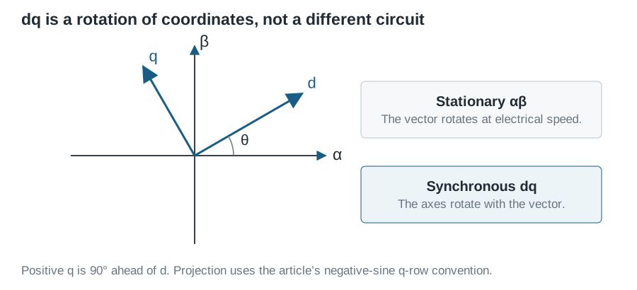
3. Rotate the axes

For the controller’s chosen angle \(\theta_r\), define the Park transform as

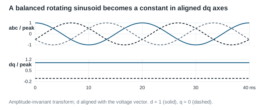
\[\begin{bmatrix}x_d\\x_q\end{bmatrix} =\underbrace{\begin{bmatrix}\cos\theta_r&\sin\theta_r\\-\sin\theta_r&\cos\theta_r\end{bmatrix}}_{T(\theta_r)} \begin{bmatrix}x_\alpha\\x_\beta\end{bmatrix}. \tag{4}\]

Thus \(x_d=X\cos(\theta-\theta_r)\) and \(x_q=X\sin(\theta-\theta_r)\). When the reference angle follows the waveform, \(x_d=X\) and \(x_q=0\). Reconstruction uses \(T^{-1}=T^T\) followed by the inverse Clarke transform. These explicit matrices prevent ambiguity: another source may use a different q direction or normalisation.

The upper traces rotate in time; the lower components remain constant only because the frame rotates at the matching angle and speed. A wrong angle produces a q component. Open full size

4. Derive the speed-coupling terms

The transformation itself changes with time. Let \(\omega_r=\dot\theta_r\). Applying the product rule gives

\[\frac{d}{dt}\begin{bmatrix}x_d\\x_q\end{bmatrix} =T\frac{d}{dt}\begin{bmatrix}x_\alpha\\x_\beta\end{bmatrix} +\omega_r\begin{bmatrix}x_q\\-x_d\end{bmatrix}. \tag{5}\]

Therefore a stationary inductor equation \(L\dot{\boldsymbol i}=\boldsymbol u-r\boldsymbol i-\boldsymbol v\) becomes

\[L\dot i_d=u_d-ri_d-v_d+\omega_rLi_q,\qquad L\dot i_q=u_q-ri_q-v_q-\omega_rLi_d. \tag{6}\]

For a capacitor with current into it equal to \(i_f-i_o\),

\[C\dot v_d=i_{f,d}-i_{o,d}+\omega_rCv_q,\qquad C\dot v_q=i_{f,q}-i_{o,q}-\omega_rCv_d. \tag{7}\]

The signs follow from differentiation; they should not be memorised independently of the matrix. In the AFE, input current is positive from source to converter, so the physical equation starts with source voltage minus converter voltage. That reversal changes the converter control sign while leaving the coordinate derivative rule unchanged.

5. Preserve power and specify reactive-power sign

The rotation preserves dot products, while the amplitude-invariant Clarke transform introduces a 3/2 scale factor. With zero sequence absent,

\[p=v_ai_a+v_bi_b+v_ci_c =\frac32(v_di_d+v_qi_q),\qquad Q=\frac32(v_qi_d-v_di_q). \tag{8}\]

For balanced sinusoidal steady state, Q is conventional reactive power with the stated current direction. A current lagging its local voltage by φ has \(i_d=I\cos\phi\) and \(i_q=-I\sin\phi\) when voltage aligns with d. Hence \(P=3VI\cos\phi/2\) and \(Q=3VI\sin\phi/2\). This gives positive Q for inductive consumption at the AFE, or positive reactive delivery for inverter current defined towards its receiving port.

Outside balanced sinusoidal operation, the instantaneous cross-product quantity must not be confused with every metering definition of reactive power. Also, power-invariant transforms use different scaling: their equations cannot be combined with the amplitudes above without conversion.

6. Where the angle comes from

A stand-alone voltage source may prescribe \(\dot\theta_r=2\pi f^*\). A grid-following converter instead estimates an existing voltage angle. Let the grid angle be \(\theta_g\) and the estimate \(\hat\theta\). The transformed grid voltage is

\[v_q=V\sin(\theta_g-\hat\theta) \approx V(\theta_g-\hat\theta). \tag{9}\]

Normalise by a suitably filtered nonzero voltage-amplitude estimate to obtain \(e\approx\theta_g-\hat\theta\). A basic synchronous-reference-frame PLL uses

\[\dot z=e,\qquad \hat\omega=\omega_0+k_pe+k_iz,\qquad \dot{\hat\theta}=\hat\omega. \tag{10}\]

A positive q voltage means the estimate is behind the source, so the controller increases estimated frequency. Linearising around lock and taking Laplace transforms gives

\[\frac{\widetilde{\hat\theta}}{\widetilde\theta_g} =\frac{k_ps+k_i}{s^2+k_ps+k_i},\qquad k_p=2\zeta\omega_n,\qquad k_i=\omega_n^2. \tag{11}\]

Tildes here denote small angle perturbations, distinguishing them from the angle-estimate hat. A tentative 20 Hz natural frequency and \(\zeta=0.707\) give \(k_p=177.7\ \mathrm{s^{-1}}\) and \(k_i=1.579\times10^4\ \mathrm{s^{-2}}\) for this normalised detector. Filtering, low-voltage handling and interaction with the current controller must be assessed before selecting actual gains.

7. Understand what the simple model leaves out

Negative sequence rotates backwards relative to the positive-sequence voltage. In a positive rotating frame it appears at twice line frequency; harmonics also remain time-varying. Unbalance therefore requires appropriate sequence extraction, resonant compensation or additional models. A dq transform alone does not remove these disturbances.

When linearising a grid-following converter, the PLL angle is also a state. Around a d-aligned operating point,

\[\widetilde v_q=-\sin\Theta_r\,\widetilde v_\alpha +\cos\Theta_r\,\widetilde v_\beta-V_d\widetilde\theta_r. \tag{12}\]

Omitting the last term hides angle coupling. Likewise, treating grid frequency as fixed is an assumption, not a property of the transform.

Verify an implementation with balanced synthetic sinusoids before connecting it to a converter model. Check that d equals the phase peak, q is zero at alignment, reconstruction returns the input and abc power equals dq power. Then impose a small positive phase step and confirm that q and the PLL’s frequency correction initially increase. These checks expose scaling and sign errors early.

For a practical example using dq voltage and current control, see Imperix’s grid-forming inverter note. Return to the series guide to place the coordinate model within the complete SST.