The forward converter ends with a complaint: its core is magnetised in one direction, then reset back to zero, and never swings negative. Only half of the available B–H loop is used. At higher power that wasted capability translates directly into a larger, heavier, more expensive transformer.

Alternating primary voltage permits a bipolar flux excursion. This can improve core utilisation for a given allowed flux-density range, but does not by itself halve core area at fixed power: turns, frequency, window utilisation and losses also matter. Equal positive and negative volt-seconds provide reset, and full-wave secondary rectification produces two energy-delivery intervals per magnetic period.

Three topologies achieve this — push–pull, half-bridge and full-bridge. They differ mainly in how many switches they use and what voltage those switches must block. All three are examined here against the same 48 V to 12 V, 30 W specification used throughout the isolated chapters, then placed in their real power ranges.

First draft — design example, not a validated reference board. Values are analytical starting points; the LTspice netlist is a teaching resource. Native simulator execution and hardware measurements are not included.

Reading route: the shared idea → push–pull → half-bridge → full-bridge → comparison → flux walking → PSFB → simulation → applications.

1. The shared idea: excite the core both ways

Every converter in this chapter does the same three things:

1. Generate an AC square wave across the transformer primary, alternating between positive and negative.
2. Rectify it on the secondary, usually with a centre-tapped winding and two diodes, or a full bridge of four.
3. Filter it with an output LC, exactly as a buck does.

Because the primary is excited twice per switching period — once positive, once negative — the rectified secondary delivers two pulses per period. The output filter therefore sees \(2f_s\), not \(f_s\). That single fact lets the output inductor and capacitor shrink by roughly half for the same ripple, and it is one of the quiet advantages of every double-ended topology.

The core also never needs a reset winding: the negative half-cycle is the reset. Volt-second balance is achieved automatically by symmetry — provided the two half-cycles really are symmetric, which is the subject of section 6.

A convention, because it causes endless confusion: in all three topologies below, \(D\) means the duty of one individual switch, which can range from 0 to 0.5. The two switches conduct in alternate half-periods, so the total conduction time is \(2D\) and the maximum is 1. Some textbooks define \(D\) as that total instead, which changes every formula by a factor of two.

2. Push–pull

These are winding-voltage waveforms, not a centre-tapped wiring schematic. A push-pull winding referenced to a fixed core polarity has alternating excitation too; its turns ratio is defined per half-primary. Open full size

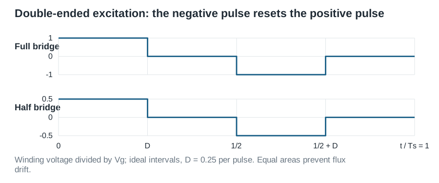
Two switches, both ground-referenced — the great practical attraction, because neither needs a floating gate drive. The primary is centre-tapped: S1 energises one half, S2 the other, producing an alternating flux.

With \(n=N_p/N_s\) defined per half-primary:

\[\boxed{V=\frac{2DV_g}{n}}. \tag{1}\]

For our example, \(n=2\) and \(D=0.25\) per switch gives \(V=12\ \mathrm{V}\).

Now the problem. When S1 conducts, its half of the primary sees \(V_g\) — but the transformer couples that same \(V_g\) into the other half, so the open switch S2 sees the input plus the coupled voltage:

\[\boxed{V_{\mathrm{DS,off}}=2V_g} \tag{2}\]

96 V for a 48 V input, before leakage overshoot. This higher switch stress is one reason push–pull is often considered for lower-voltage inputs. Device selection must use the maximum input, measured or simulated overshoot and protection limits; nominal input alone cannot justify a voltage rating.

The push–pull is also the topology most vulnerable to flux walking, because its two halves are driven by physically different switches and windings.

3. Half-bridge

This drawing isolates the Q1/Q2 switching leg. For the transformer-fed half bridge discussed here, connect the primary between this switching output and a separate split-capacitor midpoint; that midpoint and transformer are not shown in this leg-only figure. Open full size · Circuit source · Drawn with AIPE-Sketch

Two capacitors split the DC link, holding the midpoint at \(V_g/2\). The primary is connected between the switch node and that midpoint, so it sees ±\(V_g/2\):

\[\boxed{V=\frac{DV_g}{n}}. \tag{3}\]

With \(n=1\) and \(D=0.25\), that is 12 V for our example.

The payoff is decisive:

\[\boxed{V_{\mathrm{DS,off}}=V_g} \tag{4}\]

Each switch blocks only the input voltage — half the push–pull’s stress. This is why the half-bridge, not the push–pull, is the standard choice for offline supplies: a 400 V DC link needs 500–600 V devices rather than 800 V ones.

The split capacitors provide the primary return at their midpoint. Their balance and the actual positive/negative volt-seconds must still be checked, particularly during startup and unequal loading. A dedicated series DC-blocking capacitor can help constrain flux bias in suitable designs, but the split bus is not unconditional protection against flux walking. The half bridge also requires a suitable high-side drive and carries more primary current than a full bridge at equal transferred power and waveform assumptions.

4. Full-bridge

Q1/Q4 and Q2/Q3 apply opposite voltage across the AC port. R1 here marks that port with a resistive load; an isolated converter connects its transformer primary there and adds the secondary rectifier and filter. Open full size · Circuit source · Drawn with AIPE-Sketch

Four switches in two legs. Diagonal pairs conduct together: S1+S4, then S2+S3. The primary sees the full ±\(V_g\):

\[\boxed{V=\frac{2DV_g}{n}} \tag{5}\]

while each switch still blocks only

\[\boxed{V_{\mathrm{DS,off}}=V_g}. \tag{6}\]

This is the best of both: full voltage across the primary (so half the primary current of a half-bridge for the same power) and only \(V_g\) of switch stress. Like the half-bridge, it is naturally protected against flux walking if a small DC-blocking capacitor is placed in series with the primary, where the chosen design includes one; its startup and resonant effects still need analysis.

The price is four switches and two high-side drives. That overhead is irrelevant at high power, where semiconductor stress dominates the cost, which is why the full bridge owns the high-power end of isolated conversion.

5. Choosing between them

All three evaluated at 48 V → 12 V, 30 W:

	Push–pull	Half-bridge	Full-bridge
Switches	2	2	4
Primary voltage	±\(V_g\)	±\(V_g/2\)	±\(V_g\)
Switch stress	\(2V_g\) = 96 V	\(V_g\) = 48 V	\(V_g\) = 48 V
Conversion ratio	\(2DV_g/n\)	\(DV_g/n\)	\(2DV_g/n\)
Primary current	lowest	highest (2×)	lowest
Gate drives	both low-side	one high-side	two high-side
Flux-walk protection	none inherent	inherent (coupling caps)	with blocking cap
Transformer	centre-tapped primary	simple	simple
Typical power	100 W – 1 kW	150 W – 1 kW	500 W – many kW
Typical input	low voltage (12–48 V)	offline / high voltage	high power, any voltage

The decision is usually straightforward:

• Low input voltage, want simple gate drive? Push–pull. The \(2V_g\) stress is harmless at 24 V or 48 V.
• Offline or high-voltage input, moderate power? Half-bridge. Halving the switch stress matters far more than the doubled primary current.
• High power? Full bridge. Lowest combination of voltage and current stress; the extra switches pay for themselves.

Note what does not change: every one of these is a buck downstream of the rectifier, so the output-stage sizing, the small-signal plant and the compensator design follow the forward converter’s treatment exactly, with \(G_{d0}\) adjusted for the topology’s conversion ratio and the ripple frequency doubled to \(2f_s\).

The voltage is rectangular but flux is its integral. This separate 48 V, 50 kHz magnetic example illustrates the relationship; use the winding voltage and turns of your own bridge design. Open full size

6. Flux walking: the failure mode to design against

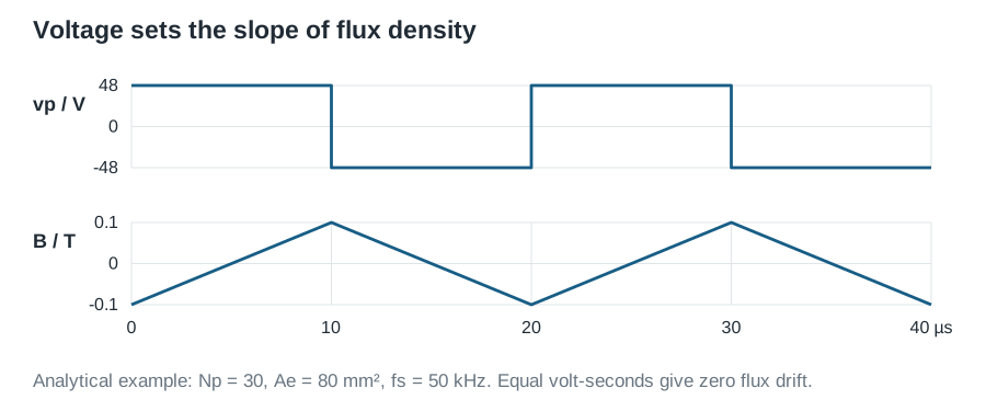
Symmetry is what resets the core, and symmetry is never perfect. If the positive half-cycle applies even slightly more volt-seconds than the negative one — because of unequal on-times, mismatched switch delays, different \(R_{\mathrm{DS(on)}}\) or asymmetric windings — the flux does not return to its starting point. The offset accumulates cycle after cycle until the core saturates, the primary inductance collapses, and the switch sees an effectively short-circuited transformer.

This happens in milliseconds and is catastrophic. Three defences are used:

1. A DC-blocking capacitor in series with the primary. Any DC voltage component develops across the capacitor instead of the winding. The half-bridge gets this free from its split capacitors; full bridges usually add one deliberately. Push–pull cannot easily use one, because its primary is centre-tapped — which is precisely why it is the most vulnerable.
2. Peak current-mode control. Terminating each pulse on a current threshold rather than a fixed time naturally equalises the two half-cycles, because a walking flux shows up as a rising current. This is the standard answer for push–pull.
3. A small core air gap. Reduces the flux excursion for a given volt-second error, trading magnetising current for margin.

If you take one practical warning from this article: never run a push–pull in open-loop voltage mode at a fixed duty, which is exactly what the supplied netlist does for teaching purposes. It is safe in simulation with ideal switches and will not be safe on the bench.

7. The phase-shifted full bridge

At higher powers, hard switching a full bridge wastes significant energy, and the natural evolution is the phase-shifted full bridge (PSFB).

Both legs run at a fixed 50 % duty. Regulation comes from shifting the phase between them: when the legs are in phase, the diagonal overlap is zero and no power transfers; as the phase shift grows, the overlap and the transferred power grow with it. Effective duty is the overlap angle.

The reason this matters is zero-voltage switching. The transformer’s leakage inductance, plus the output inductor current reflected to the primary, resonates with each switch’s output capacitance during the transition, discharging it before the device turns on. Switching loss largely disappears, allowing higher frequencies and smaller magnetics.

Two honest caveats:

• ZVS is load-dependent. The energy available to discharge the switch capacitance comes from the inductive current, so ZVS is lost at light load. The lagging leg loses it first. Designs often add a shunt inductor or accept partial hard switching at low power.
• Duty loss. Time spent commutating the leakage inductance does not deliver power, so the effective secondary duty is less than the primary phase overlap — and the shortfall grows with load current. Account for it when choosing the turns ratio, or the converter will fail to reach full output at low line.

The PSFB is the standard topology for kilowatt-class isolated DC–DC, from telecom rectifiers to EV on-board chargers. Where bidirectional flow is also required, the diode rectifier is replaced with a second active bridge, giving the dual active bridge already covered in this series.

8. Simulate it

Open halfbridge_open_loop.cir and plot V(out), V(n1), V(a), V(mid) and I(Lo).

1. V(n1) shows two pulses per switching period. The output filter sees 200 kHz from a 100 kHz converter — measure the ripple frequency directly and confirm it.
2. V(mid) sits at 24 V, half the input, confirming the split-capacitor midpoint.
3. V(a) swings between 0 and 48 V, so each switch blocks only \(V_g\) — contrast this with the 96 V a push–pull switch would see.
4. I(Lo) is a triangle on 2.5 A, exactly like a buck, but ripples at twice the switching frequency.

Two instructive modifications:

• Watch the dead time. Reduce the gap between Vg1 and Vg2 until they overlap, and both switches conduct simultaneously — a direct short across the DC link. Shoot-through is the bridge topology’s other classic failure mode, and adequate dead time is what prevents it.
• Create a flux walk. Make one gate pulse slightly longer than the other (say 2.6 µs against 2.5 µs) and watch the magnetising current drift. In this half-bridge the coupling capacitors will largely absorb it — which demonstrates their protective role better than any description.

9. Where these converters are used

Push–pull — low-voltage, moderate-power isolated supplies: 24 V and 48 V industrial rails, battery-fed inverter front ends, automotive auxiliary supplies, and isolated DC–DC modules where both gate drives being ground-referenced simplifies the design.

Half-bridge — the mainstream offline choice from roughly 150 W to 1 kW: ATX and server power supplies, industrial supplies, welding equipment, and lighting ballasts. Its descendant, the LLC resonant converter, now dominates this space by adding a resonant tank to the same half-bridge.

Full bridge and PSFB — high-power isolated conversion: telecom rectifiers, EV on-board chargers and DC fast-charging modules, industrial plating and induction supplies, and the isolation stage of larger systems. Above a few hundred watts it is usually the default.

Where not to use them. Below about 100 W the switch count, gate-drive complexity and transformer cost are not justified — a flyback or forward converter will be cheaper and smaller. And if efficiency at high frequency is the priority rather than raw power, the resonant approach in the next chapter usually beats a hard-switched bridge outright.

Further study

Robert W. Erickson and Dragan Maksimović, Fundamentals of Power Electronics, third edition, Springer, 2020, for transformer-isolated converter families and their steady-state analysis. The derivations and numerical examples here are presented independently; this article is not a reproduction of the textbook.