A lifetime estimate is a conditional prediction about a population under a defined operating history. It requires more than a switching-loss measurement, a maximum junction temperature or a qualification pass. This final chapter connects the measurements in the characterisation series to the assumptions needed for a defensible estimate.

There are two distinct descriptions to retain. A damage model relates stress exposure to degradation for a particular mechanism. A lifetime distribution describes variation between specimens. Neither replaces the other.

1. Define the mission and the event called failure

A mission profile describes how the equipment operates: load, bus voltage, switching strategy, start/stop events, ambient or coolant conditions, dwell, storage and faults. State its duration, sampling interval and the population it represents. A convenient nominal day may omit seasonal extremes or rare events that dominate damage.

Define failure before fitting life data: loss of function, a specified parameter crossing under matched conditions, or another justified application limit. Record whether the estimate concerns a die, package, module or complete converter. Several device failure mechanisms and other converter components may contribute to system failure.

2. Convert operation into the relevant stress history

Step	Model input	Result to retain
Electrical operation	Voltage, current, modulation and gate conditions	Per-device conduction and switching events
Loss calculation	Measured loss maps and parameter dependence	Time-dependent power, with interpolation limits
Thermal calculation	Validated thermal network, mounting and cooling	Junction and relevant package-temperature histories
Stress extraction	Temperature extrema, dwell, electrical field and moisture	Mechanism-specific cycles or exposure intervals
Life calculation	Calibrated damage law and specimen statistics	Conditional estimate with uncertainty

Iterate loss and temperature where their coupling matters. Use the transient thermal model rather than converting every instantaneous loss sample into a steady-state temperature. Averaging switching-period losses is appropriate only when the thermal bandwidth of interest permits it; retain slower ripple and transients that materially affect temperature.

For thermal fatigue, identify turning points in the temperature history and apply a documented cycle-counting method, such as rainflow counting. Rainflow pairs nested reversals into full or residual half cycles. State whether the bin variable is the full temperature range or its half-amplitude; confusing these changes a power-law life estimate substantially. Retain the corresponding temperature level and duration if the calibrated model uses them.

A power-cycling model does not automatically represent passive temperature cycling or humidity and gate-bias degradation. Match the model to the observed mechanism and loading.

3. Compute cumulative damage with explicit assumptions

A commonly used linear fatigue approximation is the Palmgren–Miner sum:

\[D=\sum_i\frac{n_i}{N_{f,i}}. \tag{1}\]

Here \(n_i\) is the number of applied cycles in stress bin i and \(N_{f,i}\) is the fitted life under that bin’s constant-amplitude conditions, using a consistently defined life statistic. The conventional threshold \(D=1\) is a modelling assumption. The sum ignores load-sequence effects and interactions; the damage fraction is not a probability of failure.

Consider a synthetic mission block with 1,000 cycles assigned a life of 100,000 cycles, and 100 cycles assigned a life of 10,000 cycles:

\[D_{\mathrm{block}}=\frac{1000}{100000}+\frac{100}{10000}=0.02. \tag{2}\]

The model reaches unity after 50 identical blocks. This is an arithmetic example, not a device lifetime prediction. Changing cycle order, mechanism, mission or the life statistic can invalidate that interpretation. Calendar years require a justified mapping from real operation to blocks, including periods that activate other degradation mechanisms.

4. Use acceleration only within its calibrated mechanism

For an appropriate thermally activated mechanism, an Arrhenius model relates a characteristic failure time to absolute temperature:

\[t_f(T)=A\exp\!\left(\frac{E_a}{k_BT}\right),\qquad AF=\frac{t_f(T_{\mathrm{use}})}{t_f(T_{\mathrm{test}})} =\exp\!\left[\frac{E_a}{k_B}\left(\frac1{T_{\mathrm{use}}}-\frac1{T_{\mathrm{test}}}\right)\right]. \tag{3}\]

Use kelvin, with \(k_B=8.617\times10^{-5}\ \mathrm{eV/K}\) when activation energy \(E_a\) is in electronvolts. The activation energy must describe the mechanism and materials; it is not a universal semiconductor constant. NIST’s Arrhenius model reference gives the temperature-acceleration relationship.

As a synthetic calculation, \(E_a=0.7\ \mathrm{eV}\), a 75 °C use temperature and a 125 °C test temperature give \(AF\approx18.7\). This factor assumes unchanged other stresses and mechanism. It cannot be applied wholesale to mechanical fatigue or to a combined humidity/voltage test. Validate stress dependence using multiple levels and examine failure evidence for mechanism changes.

5. Describe specimen variation with a lifetime distribution

For cycles-to-failure N, the two-parameter Weibull distribution is

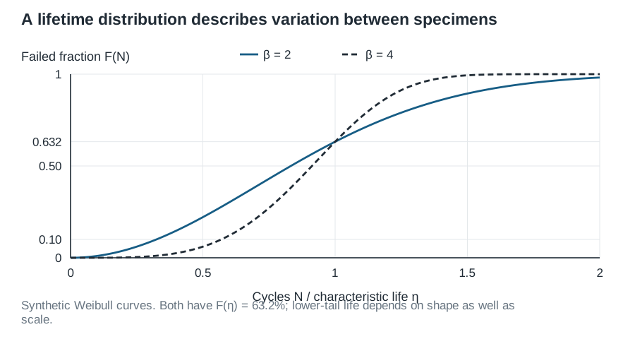
\[F(N)=1-\exp[-(N/\eta)^\beta],\qquad S(N)=1-F(N). \tag{4}\]

F is the failed population fraction and S the survival probability. The positive parameters \(\eta\) and \(\beta\) describe scale and shape. The scale corresponds to about 63.2% cumulative failures, not the mean life. For a specified failure fraction p,

\[N_p=\eta[-\ln(1-p)]^{1/\beta}. \tag{5}\]

For example, B10 life uses \(p=0.10\). A fitted B10 value and a lower confidence bound on B10 are different quantities. NIST’s Weibull reference provides the distribution and its properties. A convenient distribution fit alone does not establish the physical failure mechanism.

Both curves reach 63.2% failures at η, but their low-percentile lives differ. A characteristic life is not a guaranteed lifetime for every specimen. Open full size

6. Keep survivors and inspection intervals in the fit

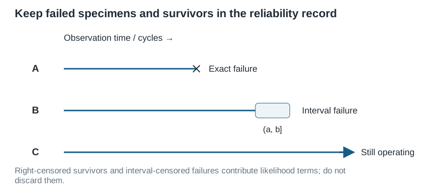
A specimen still operating when observation stops is right-censored. If failure is found only at a checkpoint, its failure time lies between the last passing and first failing inspections. These observations carry information.

For independent specimens and non-informative censoring, the parameter-dependent likelihood has contributions

\[\mathcal{L}(\theta)= \prod_{i\in\mathcal{E}} f(N_i;\theta) \prod_{j\in\mathcal{R}} S(c_j;\theta) \prod_{k\in\mathcal{I}}[F(b_k;\theta)-F(a_k;\theta)]. \tag{6}\]

Here f is the failure density, E denotes exact failures, R survivors observed to \(c_j\), and I failures in intervals \((a_k,b_k]\). Maximising this likelihood uses all three kinds of evidence; fitting only failed specimens generally biases the result. NIST’s maximum-likelihood tutorial explains this approach. Removal because a specimen appears close to failure may be informative and needs explicit treatment.

A survivor says that life exceeds its observation time. A checkpoint failure supplies an interval. Both are useful evidence and belong in the fit. Open full size

7. Understand what zero failures establish

Suppose n independent, representative specimens all survive the same exposure. At a hypothetical survival probability R, the probability of that observation is \(R^n\). Solving \(R_L^n=\alpha\) gives the exact one-sided lower confidence bound

\[R_L=\alpha^{1/n},\qquad \text{confidence level}=1-\alpha. \tag{7}\]

For 30 survivors and 95% confidence, \(R_L=0.05^{1/30}\approx0.905\). The bound concerns survival through that particular exposure under the sampling assumptions. It does not establish 100% reliability, a Weibull shape or a number of field years. Correlated specimens or a narrowly selected lot reduce the scope of the inference.

8. Report a prediction that can be challenged

Validate the model on stress levels, waveforms or samples not used to fit it. Carry uncertainty from the mission, loss maps, temperature measurement, thermal model, acceleration parameters and specimen variation. Statistical confidence in a fitted curve does not include all model error.

Report the population, mechanism, failure criterion, exposure domain, life statistic and uncertainty together. Keep competing mechanisms separate unless a justified combined model is available. The final engineering result is a conditional prediction with evidence that can be traced back to measurements, not a single unsupported lifespan number.