
Thermal resistance appears simple: divide temperature rise by dissipated power. The difficulty is establishing which temperature, which power and which heat-flow path belong in that division. Without those definitions, two plausible measurements can describe different systems.
Read the junction-temperature tutorial first. This chapter then establishes the steady-state boundary used by the transient model.
1. Define the thermal ports
For an approximately linear heat-flow path under a specified boundary condition,
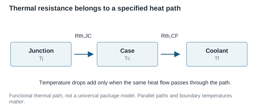
\[R_{\mathrm{th},j-r}=\frac{T_j-T_r}{P_{\mathrm{path}}}. \tag{1}\]The reference r might be a defined case surface, a controlled cold plate or ambient air. Heat flowing through the path is \(P_{\mathrm{path}}\). It equals total device dissipation only when other heat-flow paths are negligible or when the specified test method defines an effective metric using total power.
Datasheet thermal metrics belong to their measurement conventions:
| Metric | Interpretation |
|---|---|
| Junction-to-case resistance | A specified junction-to-case path and boundary; the relevant case surface must be identified |
| Junction-to-ambient resistance | Effective behaviour of a device mounted and cooled in a stated environment, often including a specified PCB |
| Junction-to-board resistance | Behaviour defined using a particular board reference and measurement procedure |
| Thermal characterisation parameter, such as ψJT | A temperature difference divided by total power under a specified test; generally not an independent physical branch resistance |
A heatsink attached to the top of a dual-side-cooled device can change how heat divides between paths. The measured top temperature difference divided by total power cannot then automatically be used as the resistance carrying all heat to that surface.
2. Control the mechanical and cooling boundary
Specify the mounting surface, flatness, thermal interface material (TIM), thickness or application method, pressure/torque, cold-plate temperature and coolant flow. For a PCB-cooled device, copper area, layers, vias and airflow are part of the test article.
Place the reference sensor at the defined location without substantially disturbing contact. A hole, thick thermocouple bead or uneven TIM can change the quantity being measured. A coolant inlet temperature is not necessarily the local case or cold-plate surface temperature.
Let the device reach an identified equilibrium condition, based on observed temperature slopes and power stability. State the criterion and hold time selected for the experiment rather than assuming that an arbitrary wait guarantees equilibrium.
3. Measure dissipation at the DUT boundary
Conduction heating can simplify the experiment because power is obtained from simultaneous terminal voltage and current:
\[P_H=\langle v_D(t)i_D(t)\rangle. \tag{2}\]Do not use supply power without separating losses in cables, shunts and other series devices. With pulsed or switched excitation, average the instantaneous product over the relevant interval; the product of average voltage and average current may be different.
Account for sensing-power and gate-drive contributions if they matter to the uncertainty target. If electrical heating is uneven across multiple dies, the inferred junction temperature and thermal resistance may depend on the current distribution.
4. Acquire a power-versus-temperature curve
First record the zero-heating reference state. Apply several non-destructive heating levels, maintaining the same boundary, and obtain \(T_j\) using the calibrated method. If heating must be interrupted for sensing, correct or bound the associated cooling error.
Plot temperature rise against dissipated power:
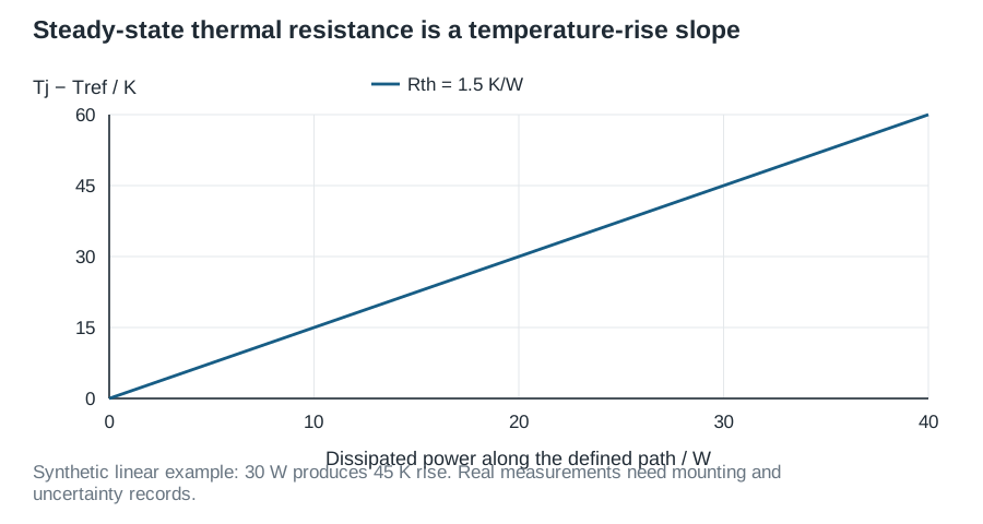
\[T_j-T_r\approx R_{\mathrm{th}}P_H+b. \tag{3}\]A nonzero intercept b can indicate temperature-reference offsets or other heat sources. Curvature can indicate temperature-dependent properties or a cooling boundary that changes with power. Do not force a linear fit over a range that contradicts the data.
In a synthetic example, 30 W produces a 45 K junction-to-reference rise:
\[R_{\mathrm{th}}=45/30=1.50\ \mathrm{K/W}. \tag{4}\]This number has no useful package meaning until the reference location and heat-flow assumptions are stated.
5. Separate the interface from the package
For an approximately one-dimensional series path with negligible parallel heat flow,
\[R_{j-\mathrm{sink}}\approx R_{j-c}+R_{c-\mathrm{sink}}. \tag{5}\]Subtracting measurements to isolate a small interface resistance amplifies uncertainty and assumes the other paths remain unchanged. Re-mounting may alter pressure, contact area or TIM distribution, so repeat mounts as part of the repeatability study.
Transient dual-interface methods compare two controlled case-to-cooler boundary conditions to help identify the junction-to-case portion of the response. Their validity depends on the method’s package and heat-flow assumptions. Siemens’ explanation of the JESD51-14 approach gives context; following a simplified sketch is not a claim of performing the complete standard.
6. Quantify uncertainty and repeatability
For independent temperature-rise and power uncertainties,
\[\left(\frac{u_R}{R}\right)^2\approx \left(\frac{u_{\Delta T}}{\Delta T}\right)^2+ \left(\frac{u_P}{P}\right)^2. \tag{6}\]With 45 K rise, 30 W power, \(u_{\Delta T}=1\ \mathrm K\) and \(u_P=0.3\ \mathrm W\), the illustrative standard uncertainty is approximately 0.037 K/W. Contact variability, thermal nonuniformity and calibration covariance may increase the complete budget.
Measure repeatability without moving the device, then repeat after re-mounting. These answer different questions: instrument stability and assembly reproducibility. For a cooling-interface comparison, assembly reproducibility may dominate.
7. Use the result within its measured domain
For steady operation, a first temperature estimate is \(T_j\approx T_r+P_HR_{\mathrm{th}}\). Iterate if power depends strongly on temperature. Do not replace the transient impedance by its steady resistance for short pulses, or transplant a junction-to-ambient value from one PCB to a different assembly without checking the change.
The report should include the fixture drawing, power boundary, temperature method, equilibrium evidence, repeat mounts, fit residuals and uncertainty. Those details make the measurement a reusable engineering input rather than an isolated number.