
A device dissipating a short pulse does not immediately reach its steady temperature rise. Heat spreads through the die, attachment, package and cooling system over different timescales. Transient thermal impedance describes that response under specified boundary conditions.
This article builds on junction-temperature measurement and steady thermal resistance. It connects measured temperature histories to the models needed for pulse heating and mission-profile analysis.
1. Define a step response
Assume an approximately linear, time-invariant thermal system, initially at equilibrium, with a fixed reference temperature. Apply a constant heating-power step P0 at time zero. Define
\[Z_{\mathrm{th}}(t)=\frac{T_j(t)-T_{\mathrm{ref}}}{P_0},\qquad R_{\mathrm{th}}=\lim_{t\to\infty}Z_{\mathrm{th}}(t). \tag{1}\]Z has units K/W. It is a time-domain step response, not the electrical switching impedance of the device. If coolant temperature changes during the experiment, it is another input to the thermal system; subtracting an arbitrary changing surface temperature does not necessarily recover the fixed-boundary response.
2. Measure heating or cooling with a known history
A heating measurement observes the rise after power application. A cooling measurement heats the device, removes heating power and uses a low-power TSEP to observe the decay. Cooling often makes electrical sensing easier, but the initial heating duration must be known.
For heating held long enough to reach equilibrium, followed by switch-off at time zero,
\[T_{j,\mathrm{cool}}(t)-T_{\mathrm{ref}} =P_0[R_{\mathrm{th}}-Z_{\mathrm{th}}(t)]. \tag{2}\]Only under this initial steady-state condition can the cooling curve be complemented directly into the heating step response. If heating lasted a finite duration th, superposition instead gives, at time t after switch-off,
\[T_{j,\mathrm{cool}}(t)-T_{\mathrm{ref}} =P_0[Z_{\mathrm{th}}(t+t_h)-Z_{\mathrm{th}}(t)]. \tag{3}\]Record heating voltage/current, heating duration, switching-to-sensing delay and the first trustworthy reading. Early electrical artefacts and the blind interval must be assessed before fitting fast thermal modes.
3. Derive a single thermal RC response
For a lumped thermal capacitance Cth connected to a fixed reference through Rth,
\[C_{\mathrm{th}}\frac{d\Delta T}{dt}=P_0-\frac{\Delta T}{R_{\mathrm{th}}}. \tag{4}\]With zero initial rise, the solution is
\[Z_{\mathrm{th}}(t)=R_{\mathrm{th}}(1-e^{-t/\tau}),\qquad \tau=R_{\mathrm{th}}C_{\mathrm{th}}. \tag{5}\]Cth has units J/K. The thermal analogy uses temperature as voltage and heat flow as current. One time constant rarely represents the complete package and cooler over many decades of time.
4. Fit several time constants without inventing physical layers
A Foster representation of a collocated heating/temperature response is commonly written
\[Z_{\mathrm{th}}(t)=\sum_{k=1}^{m}R_k(1-e^{-t/\tau_k}), \qquad R_k>0,\quad \tau_k>0. \tag{6}\]Positive parameters give a monotonic step response for this model. Each \(C_k=\tau_k/R_k\) is a model parameter. A Foster branch does not automatically correspond to die, solder or baseplate; the internal nodes are not generally physical interface temperatures.
A Cauer ladder has a different network structure and is better suited to physically meaningful boundary connections when derived and validated appropriately. Do not attach a heatsink model to an arbitrary internal Foster node. Transformations and fitting can be numerically sensitive, and a good terminal fit does not guarantee a unique physical layer interpretation.
Fit over the measured time range with appropriate weighting. Uniform weighting on densely sampled long-time data can hide early-time error. Use the simplest model that meets the required predictive accuracy, inspect residuals and preserve uncertainty in poorly resolved time constants. Structure functions can help compare heat paths, but interface identification needs independent structural evidence.
5. Predict temperature for arbitrary power
Define the impulse response \(h(t)=dZ_{\mathrm{th}}/dt\). Then
\[\Delta T_j(t)=\int_0^t h(t-\tau)P(\tau)\,d\tau. \tag{7}\]For a piecewise-constant power sequence expressed as steps \(\Delta P_r\) at times tr,
\[\Delta T_j(t)=\sum_r\Delta P_rZ_{\mathrm{th}}(t-t_r), \qquad Z_{\mathrm{th}}(t)=0\text{ for }t<0. \tag{8}\]A rectangular pulse is one positive step and one negative step. Include previous pulses until the periodic temperature history converges; multiplying average power by steady resistance misses cyclic peaks. onsemi’s thermal application note discusses transient thermal response and its use in estimating junction temperature.
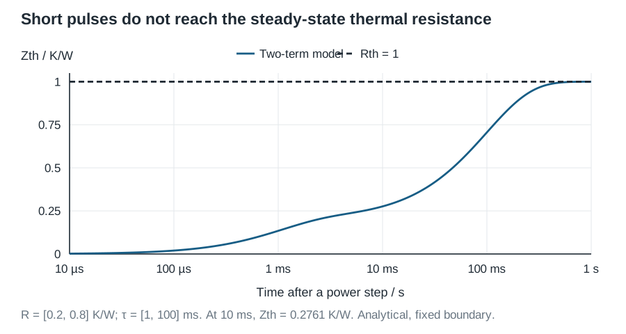
Consider a synthetic two-term model: \(R_1=0.2\ \mathrm{K/W}\), \(\tau_1=1\ \mathrm{ms}\), \(R_2=0.8\ \mathrm{K/W}\) and \(\tau_2=100\ \mathrm{ms}\). At 10 ms,
\[Z_{\mathrm{th}}(10\ \mathrm{ms})\approx0.2761\ \mathrm{K/W}. \tag{9}\]A 50 W pulse starting from equilibrium therefore produces about 13.81 K rise at its 10 ms end. Its steady 50 K rise would require sustained heating. This example demonstrates model use, not a specific device’s thermal performance.
6. Extend carefully to multiple heat sources
In a module with several dies, one die’s dissipation can heat another. A linear multi-source model is
\[\Delta T_i(t)=\sum_j\int_0^t h_{ij}(t-\tau)P_j(\tau)\,d\tau. \tag{10}\]Self-heating and cross-heating responses require separate excitations or a justified identification method. Do not assume every die sees the same temperature or that a single shared resistance captures transient coupling.
7. Validate outside the fitting experiment
Fit using one step experiment, then predict pulses of other durations and a repeated pulse sequence without refitting. Compare peak temperature, recovery and the long-time limit. Repeat at another power and base temperature to test the assumed linearity.
Record mounting, cooling, calibration, time resolution, delay corrections and the complete power history. If material properties or cooling vary materially with temperature, use a temperature-dependent or nonlinear model. The purpose is reliable prediction within a defined domain, not obtaining the largest possible number of RC branches.