
Power cycling repeatedly heats a semiconductor using its own losses and allows it to cool. Differences in thermal expansion between materials create repeated mechanical strain. Interconnects, attachment layers and other parts of the package can deteriorate, while electrical bias may activate additional mechanisms.
A count of applied pulses is insufficient to define the experiment. The actual junction-temperature history, heating duration, cooling boundary and electrical loading determine the stress. This chapter follows the baseline electrical and thermal measurements in the series guide.
1. Define a cycle by its measured stress
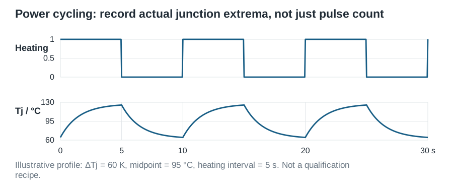
For a recorded cycle, define
\[\Delta T_j=T_{j,\max}-T_{j,\min},\qquad T_{j,\mathrm{mid}}=\frac{T_{j,\max}+T_{j,\min}}2. \tag{1}\]The midpoint is not necessarily the time-average temperature for an asymmetric waveform. Report both when the chosen life model requires them. Also record heating/cooling durations, current, voltage, case temperature and any dwell at high temperature.
A short pulse mainly heats the die and nearby structures. Longer cycles can involve a larger fraction of the package and cooling assembly. Equal junction-temperature swing with different durations does not guarantee equal strain or failure mechanisms.
2. Choose the heating method and control policy
Conduction heating can provide a controlled pulse of loss; application-like switching cycles can reproduce additional electrical stress. A published AC power-cycling study illustrates the latter and its condition-monitoring requirements. The chosen heating method belongs in the test definition.
Two common policies answer different questions:
| Policy | What is held fixed | What can change during ageing |
|---|---|---|
| Fixed electrical/timing programme | Applied current and pulse timing, within limits | Actual power and temperature excursion as device parameters drift |
| Regulated thermal programme | Selected junction-temperature endpoints or excursion | Current, power or timing needed to maintain those targets |
Neither policy should be described only as a fixed temperature swing unless that swing is measured and maintained. A feedback controller can conceal degradation by reducing applied power; its commands must be logged alongside temperature.
3. Establish the baseline and monitoring chain
Identify samples and lots, document mounting, and measure pre-stress on-state parameters, leakage and thermal response. Calibrate the selected TSEP over the intended range. If the TSEP itself ages, arrange independent checks or recalibration so that thermometer drift is not interpreted as device heating.
During cycling, log the actual temperature extrema, current, power, timing and protective interruptions. Inspect representative waveforms, not only summary values. Compare samples at matched stress and reference conditions.
At planned checkpoints, repeat electrical and thermal measurements after a specified recovery interval. For a monitored parameter x, record
\[\delta_x(N)=\frac{x(N)-x(0)}{x(0)}. \tag{2}\]On-state voltage measured at a hotter temperature is not direct evidence of ageing. Correcting it with an assumed temperature coefficient also introduces uncertainty. Preserve the raw measurement and the correction separately.
4. Connect indicators to physical mechanisms
Changes in on-state voltage, resistance or thermal impedance can indicate interconnect or attachment degradation, but a single indicator rarely identifies the mechanism uniquely. Gate-parameter drift can instead reflect trapping or dielectric changes. Contact resistance in the fixture can imitate a DUT change.
Use controlled reference measurements and physical analysis such as appropriate imaging, cross-sectioning or bond/interconnect inspection to test the mechanism hypothesis. Record whether a failure originated in the device, mounting, fixture or protection system.
Define termination and failure criteria before the test. These may include an application-specific electrical limit, a verified thermal change or loss of function. There is no universal percentage drift or cycle count suitable for every technology and package.
5. Retain failures and survivors in the analysis
Record cycles to the first confirmed criterion crossing. If failure is only detected between inspections, it is interval-censored between the last passing and first failing observations. A device still operating when the test stops is right-censored; it must not be counted as failed at the stopping cycle or discarded.
The lifetime-estimation chapter explains statistical distributions and mission-profile damage. One stress level can compare samples under that condition, but does not identify a general acceleration model.
6. Design a stress matrix that can support the question
Vary temperature excursion, temperature level and heating duration deliberately while controlling confounding variables. Use multiple samples and enough replication to expose specimen variation. Excessive acceleration can activate a different failure mechanism, invalidating extrapolation to service.
An illustrative fatigue relation might be
\[N_f=A(\Delta T_j)^{-m}. \tag{3}\]A and m are fitted, package- and mechanism-dependent parameters, not universal constants. At fixed other stress variables this model can describe a trend; it cannot replace the missing temperature, duration and mechanism dependence of a complete model.
Document changes in the controlled stress as specimens age. Compare the resulting failure evidence with passive temperature cycling, which heats the assembly externally and can produce different gradients. Test cycles become useful life data only when the loading and the resulting damage are both understood.